Lambert’s Projection
Lambert Conformal Conic Projection is a conical projection used widely in aviation charts. It preserves angles and shapes, providing accurate direction and distance over large areas. It is especially useful for flight planning in mid-latitude regions.
Lambert’s Modification
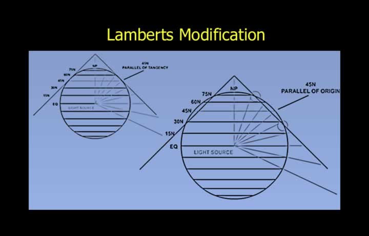
- Lambert’s projection is a non-perspective, orthomorphic (conformal), modified conical projection.
- In this projection, the cone is mathematically adjusted to pass inside the Reduced Earth.
- The parallel of origin therefore lies inside the Reduced Earth.
- The cone touches the Reduced Earth at two standard parallels.
Advantages of Lambert’s Modification
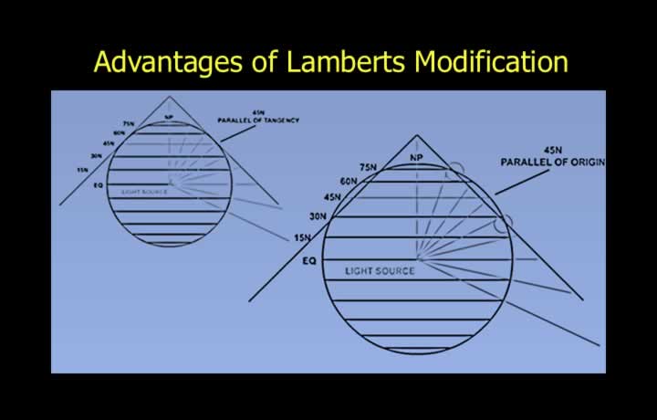
- The simple conical projection is modified to provide accurate mapping over a wider range of latitudes.
- Scale distortion is reduced to less than 1% over a much larger latitude coverage.
Lambert’s Standard Parallels
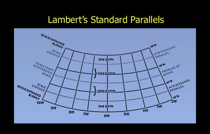
- Lambert’s projection has two standard parallels.
- The standard parallels are the latitudes where the cone touches the Reduced Earth.
- Scale is correct along both standard parallels.
- The two standard parallels and the parallel of origin divide the projection into four zones.
- The spacing of these zones is in the ratio 1 : 2 : 2 : 1.
Scale Variation in Lambert’s Projection
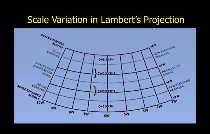
- Scale contracts between the two standard parallels.
- The minimum scale occurs at the parallel of origin.
- Scale expands outside the standard parallels.
- The greatest scale expansion occurs near the edges of the projection.
Constant Scale Chart
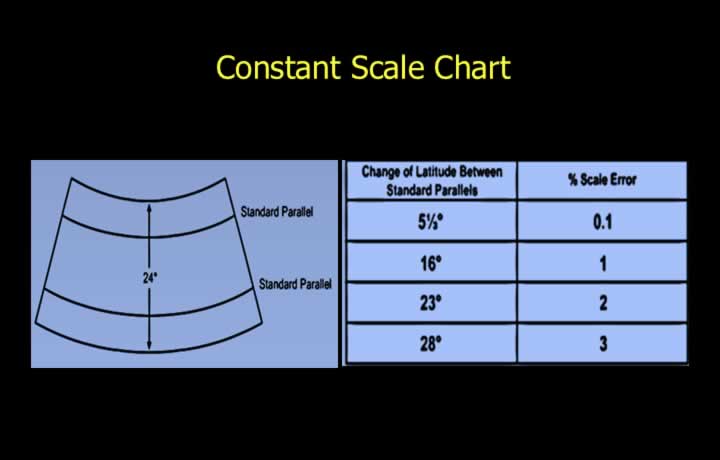
- Lambert’s projection is considered a constant scale chart under the following conditions:
- The two standard parallels are within 16° of each other.
- The chart limits extend no more than 24° beyond the standard parallels.
- Under these conditions, scale error remains within 1%.
- Distance calculations normally do not require local scale corrections.
Orthomorphism
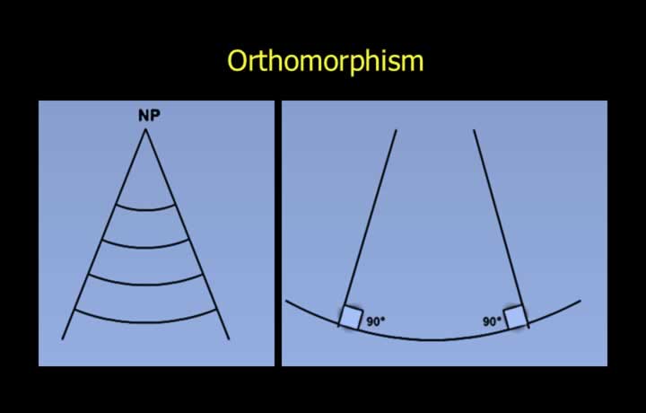
- Lambert’s projection is orthomorphic (conformal).
- Meridians are straight lines converging toward the poles.
- Parallels of latitude are arcs of circles centered on the poles.
- Meridians and parallels intersect at 90°.
Parallels and Meridians in Lambert’s Projection
- Scale expansion or contraction is the same in every direction around a point.
- North-south and east-west scales change at the same rate.
- Rhumb lines appear as curves concave toward the nearer pole.
- Parallels of latitude follow the same curvature as rhumb lines.
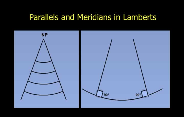
- Meridians are straight lines converging at the poles.
Earth Convergence
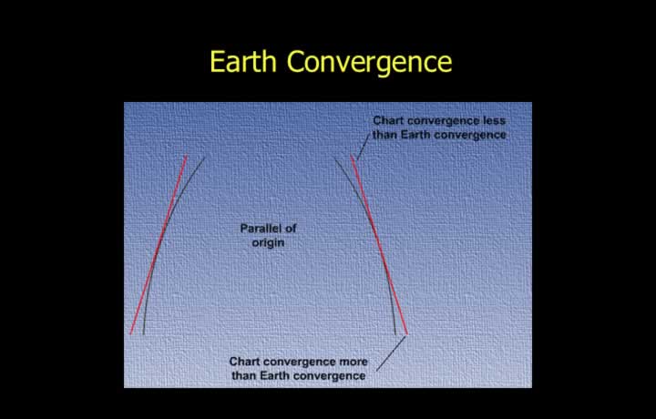
- Earth convergence is the angle between two meridians at a specified latitude.
- It represents the change in great-circle track caused by converging meridians.
- Earth Convergence = Change in Longitude × sin(Latitude)
- Earth convergence and chart convergence are equal at the parallel of origin.
Chart Convergence
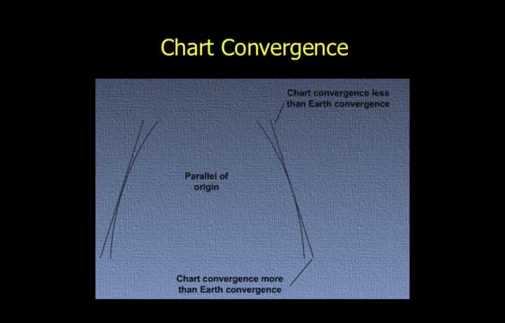
- Chart convergence is the angle between two meridians on the projection.
- It represents the change in direction of a straight line drawn on the chart.
- The straight line is neither a true great circle nor a rhumb line.
- Chart Convergence = Change in Longitude × Cone Constant
- Chart Convergence = Change in Longitude × sin(Latitude of Origin)
Earth and Chart Convergence
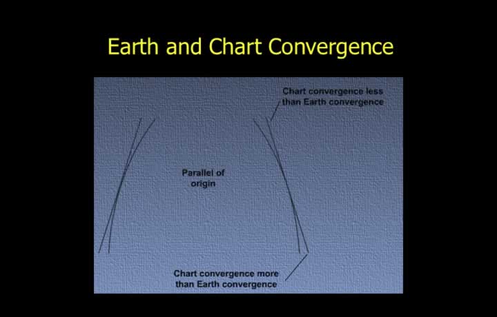
- Earth convergence and chart convergence are equal at the parallel of origin.
- Near the poles, chart convergence is less than Earth convergence.
- Near the equator, chart convergence is greater than Earth convergence.
Half Chart Convergence
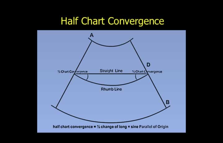
- Half chart convergence is the angular difference between a rhumb line and a straight line on the chart.
- It remains constant throughout the Lambert projection.
- Half Chart Convergence = ½ × Change in Longitude × Cone Constant
Conversion Angle vs. Half Chart Convergence
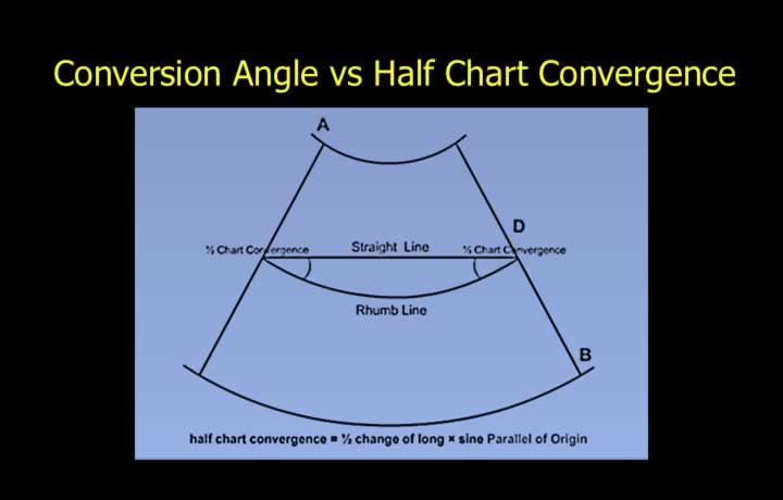
- The conversion angle is the angular difference between a rhumb line and a great-circle track.
- Unlike half chart convergence, the conversion angle varies with latitude.
- Conversion Angle = ½ × Change in Longitude × sin(Latitude)
- On a Lambert chart, great circles are concave toward the parallel of origin.
- At the parallel of origin, the conversion angle is equal to half chart convergence.
- Near the equator, the conversion angle is less than half chart convergence.
- Near the poles, the conversion angle is greater than half chart convergence.